Map Projection

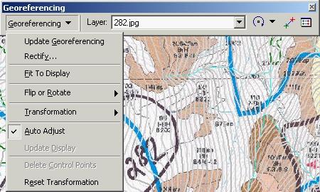
       It is impossible to accurately represent the spherical surface of the earth on a flat piece of paper. While a globe can represent the planet accurately, a globe large enough to display most features of the earth at a usable scale would be too large to be useful, so we use maps. Also imagine peeling an orange and pressing the orange peel flat on a table - the peel would crack and break as it was flattened because it can't easily transform from a sphere to a plane. The same is true for the surface of the earth and that's why we use map projections.

The term map projection can be thought of literally as a projection. If we were to place a light bulb inside a translucent globe and project the image onto a wall - we'd have a map projection. However, instead of projecting a light, cartographers use mathematical formulas to create projections.

Depending on the purpose of a map, the cartographer will attempt to eliminate distortion in one or several aspects of the map. Remember that not all aspects can be accurate so the map maker must choose which distortions are less important than the others. The map maker may also choose to allow a little distortion in all four of these aspects to produce the right type of map.

Conformality - the shapes of places are accurate

Distance - measured distances are accurate

Area/Equivalence - the areas represented on the map are proportional to their area on the earth

Direction - angles of direction are portrayed accurately

A very famous projection is the Mercator Map.

Mercator

       Geradus Mercator invented his famous projection in 1569 as an aid to navigators. On his map, lines of latitude and longitude intersect at right angles and thus the direction of travel - the rhumb line - is consistent. The distortion of the Mercator Map increases as you move north and south from the equator. On Mercator's map Antarctica appears to be a huge continent that wraps around the earth and Greenland appears to be just as large as South America although Greenland is merely one-eighth the size of South America. Mercator never intended his map to be used for purposes other than navigation although it became one of the most popular world map projections.

During the 20th century, the National Geographic Society, various atlases, and classroom wall cartographers switched to the rounded Robinson Projection. The Robinson Projection is a projection that purposely makes various aspects of the map sightly distorted to produce an attractive world map. Indeed, in 1989, seven North American professional geographic organizations (including the American Cartographic Association, National Council for Geographic Education, Association of American Geographers, and the National Geographic Society) adopted a resolution that called for a ban on all rectangular coordinate maps due to their distorion of the planet. .

                                                     Robinson Projection

 

Sources of GPS signal errors

     Factors that can degrade the GPS signal and thus affect accuracy include the following:Ionosphere and troposphere delays - The satellite signal slows as it passes through the atmosphere.     

     The GPS system uses a built-in model that calculates an average amount of delay to partially correct for this type of error.

     Signal multipath - This occurs when the GPS signal is reflected off objects such as tall buildings or large rock surfaces before it reaches the receiver. This increases the travel time of the signal, thereby causing errors.

     Receiver clock errors - A receiver's built-in clock is not as accurate as the atomic clocks onboard the GPS satellites. Therefore, it may have very slight timing errors.

     Orbital errors - Also known as ephemeris errors, these are inaccuracies of the satellite's reported location.

     Number of satellites visible - The more satellites a GPS receiver can "see," the better the accuracy. buildings, terrain, electronic interference, or sometimes even dense foliage can block signal reception, causing position errors or possibly no position reading at all. GPS units typically will not work indoors, underwater or underground.

     Satellite geometry/shading - This refers to the relative position of the satellites at any given time. Ideal satellite geometry exists when the satellites are located at wide angles relative to each other. Poor geometry results when the satellites are located in a line or in a tight grouping.

Intentional degradation of the satellite signal - Selective Availability (SA) is an intentional degradation of the signal once imposed by the U.S. Department of Defense. SA was intended to prevent military adversaries from using the highly accurate GPS signals. The government turned off SA in May 2000, which significantly improved the accuracy of civilian GPS receivers.

Source by  http://www8.garmin.com/aboutGPS/ 

What's the signal?

     GPS satellites transmit two low power radio signals, designated L1 and L2. Civilian GPS uses the L1 frequency of 1575.42 MHz in the UHF band. The signals travel by line of sight, meaning they will pass through clouds, glass and plastic but will not go through most solid objects such as buildings and mountains.

     A GPS signal contains three different bits of information - a pseudorandom code, ephemeris data and almanac data. The pseudorandom code is simply an I.D. code that identifies which satellite is transmitting information. You can view this number on your Garmin GPS unit's satellite page, as it identifies which satellites it's receiving.

     Ephemeris data, which is constantly transmitted by each satellite, contains important information about the status of the satellite (healthy or unhealthy), current date and time. This part of the signal is essential for determining a position.

     The almanac data tells the GPS receiver where each GPS satellite should be at any time throughout the day. Each satellite transmits almanac data showing the orbital information for that satellite and for every other satellite in the system.

Source by  http://www8.garmin.com/aboutGPS/ 

The GPS satellite system

     The 24 satellites that make up the GPS space segment are orbiting the earth about 12,000 miles above us. They are constantly moving, making two complete orbits in less than 24 hours. These satellites are travelling at speeds of roughly 7,000 miles an hour.

     GPS satellites are powered by solar energy. They have backup batteries onboard to keep them running in the event of a solar eclipse, when there's no solar power. Small rocket boosters on each satellite keep them flying in the correct path.

     Here are some other interesting facts about the GPS satellites (also called NAVSTAR, the official U.S. Department of Defense name for GPS):The first GPS satellite was launched in 1978.

     A full constellation of 24 satellites was achieved in 1994.

Each satellite is built to last about 10 years. Replacements are constantly being built and launched into orbit.

     A GPS satellite weighs approximately 2,000 pounds and is about 17 feet across with the solar panels extended.

     Transmitter power is only 50 watts or less.

Source by  http://www8.garmin.com/aboutGPS/ 

How accurate is GPS?

     Today's GPS receivers are extremely accurate, thanks to their parallel multi-channel design. Garmin's 12 parallel channel receivers are quick to lock onto satellites when first turned on and they maintain strong locks, even in dense foliage or urban settings with tall buildings. Certain atmospheric factors and other sources of error can affect the accuracy of GPS receivers. Garmin® GPS receivers are accurate to within 15 meters on average.

     Newer Garmin GPS receivers with WAAS (Wide Area Augmentation System) capability can improve accuracy to less than three meters on average. No additional equipment or fees are required to take advantage of WAAS. Users can also get better accuracy with Differential GPS (DGPS), which corrects GPS signals to within an average of three to five meters. The U.S. Coast Guard operates the most common DGPS correction service. This system consists of a network of towers that receive GPS signals and transmit a corrected signal by beacon transmitters. In order to get the corrected signal, users must have a differential beacon receiver and beacon antenna in addition to their GPS. 

Source by  http://www8.garmin.com/aboutGPS/ 

How it works

     GPS satellites circle the earth twice a day in a very precise orbit and transmit signal information to earth. GPS receivers take this information and use triangulation to calculate the user's exact location. Essentially, the GPS receiver compares the time a signal was transmitted by a satellite with the time it was received. The time difference tells the GPS receiver how far away the satellite is. Now, with distance measurements from a few more satellites, the receiver can determine the user's position and display it on the unit's electronic map.

     A GPS receiver must be locked on to the signal of at least three satellites to calculate a 2D position (latitude and longitude) and track movement. With four or more satellites in view, the receiver can determine the user's 3D position (latitude, longitude and altitude). Once the user's position has been determined, the GPS unit can calculate other information, such as speed, bearing, track, trip distance, distance to destination, sunrise and sunset time and more.

Source by  http://www8.garmin.com/aboutGPS/ 

What is GPS?

     The Global Positioning System (GPS) is a satellite-based navigation system made up of a network of 24 satellites placed into orbit by the U.S. Department of Defense. GPS was originally intended for military applications, but in the 1980s, the government made the system available for civilian use. GPS works in any weather conditions, anywhere in the world, 24 hours a day. There are no subscription fees or setup charges to use GPS.



Source by  http://www8.garmin.com/aboutGPS/ 

What can you do with GIS

Map Where Things Are

Mapping where things are lets you find places that have the features you're looking for and to see patterns.

Map Quantities

People map quantities to find places that meet their criteria and take action. A children's clothing company might want to find ZIP Codes with many young families with relatively high income. Public health officials might want to map the numbers of physicians per 1,000 people in each census tract to identify which areas are adequately served, and which are not.

Map Densities

A density map lets you measure the number of features using a uniform areal unit so you can clearly see the distribution. This is especially useful when mapping areas, such as census tracts or counties, which vary greatly in size. On maps showing the number of people per census tract, the larger tracts might have more people than smaller ones. But some smaller tracts might have more people per square mile—a higher density.

Find What's Inside

Use GIS to monitor what's happening and to take specific action by mapping what's inside a specific area. For example, a district attorney would monitor drug-related arrests to find out if an arrest is within 1,000 feet of a school--if so, stiffer penalties apply.

Find What's Nearby

GIS can help you find out what's occurring within a set distance of a feature by mapping what's nearby.

Map Change

Map the change in an area to anticipate future conditions, decide on a course of action, or to evaluate the results of an action or policy. By mapping where and how things move over a period of time, you can gain insight into how they behave. For example, a meteorologist might study the paths of hurricanes to predict where and when they might occur in the future.

History of GPS

    The design of GPS is based partly on similar ground-based radio-navigation systems, such as LORAN and the Decca Navigator developed in the early 1940s, and used during World War II. In 1956, Friedwardt Winterberg proposed a test of general relativity (for time slowing in a strong gravitational field) using accurate atomic clocks placed in orbit inside artificial satellites. (To achieve accuracy requirements, GPS uses principles of general relativity to correct the satellites' atomic clocks.) Additional inspiration for GPS came when the Soviet Union launched the first man-made satellite, Sputnik in 1957. Two American physicists, William Guier and George Weiffenbach, at Johns Hopkins's Applied Physics Laboratory (APL), decided on their own to monitor Sputnik's radio transmissions. They soon realized that, because of the Doppler effect, they could pinpoint where the satellite was along its orbit from the Doppler shift. The Director of the APL gave them access to their brand new UNIVAC II to do the heavy calculations required. When they released the orbit of Sputnik to the media the Russians were dumbfounded to learn how powerful American computers had become, as they would not have been able to calculate the orbit themselves. The following spring, Frank McClure, the deputy director of the APL, asked Guier and Weiffenbach to look at the inverse problem where you know the location of the satellite and you want to find your own location. (The Navy was developing the submarine launched Polaris missile, which required them to know the submarine's location.) This led them and APL to develop the Transit system.

Official logo for NAVSTAR GPS		Emblem of the 50th Space Wing

    The first satellite navigation system, Transit (satellite), used by the United States Navy, was first successfully tested in 1960. It used a constellation of five satellites and could provide a navigational fix approximately once per hour. In 1967, the U.S. Navy developed the Timation satellite that proved the ability to place accurate clocks in space, a technology required by GPS. In the 1970s, the ground-based Omega Navigation System, based on phase comparison of signal transmission from pairs of stations, became the first worldwide radio navigation system. Limitations of these systems drove the need for a more universal navigation solution with greater accuracy.
    While there were wide needs for accurate navigation in military and civilian sectors, almost none of those were seen as justification for the billions of dollars it would cost in research, development, deployment, and operation for a constellation of navigation satellites. During the Cold War arms race, the nuclear threat to the existence of the United States was the one need that did justify this cost in the view of the United States Congress. This deterrent effect is why GPS was funded. It is also the reason for the ultra secrecy at that time. The nuclear triad consisted of the United States Navy's submarine-launched ballistic missiles (SLBMs) along with United States Air Force (USAF) strategic bombers and intercontinental ballistic missiles (ICBMs). Considered vital to the nuclear deterrence posture, accurate determination of the SLBM launch position was a force multiplier.
    Precise navigation would enable United States submarines to get an accurate fix of their positions prior to launching their SLBMs. The USAF with two-thirds of the nuclear triad also had requirements for a more accurate and reliable navigation system. The Navy and Air Force were developing their own technologies in parallel to solve what was essentially the same problem. To increase the survivability of ICBMs, there was a proposal to use mobile launch platforms (such as Russian SS-24 and SS-25) and so the need to fix the launch position had similarity to the SLBM situation.
    In 1960, the Air Force proposed a radio-navigation system called MOSAIC (MObile System for Accurate ICBM Control) that was essentially a 3-D LORAN. A follow-on study called Project 57 was worked in 1963 and it was "in this study that the GPS concept was born." That same year the concept was pursued as Project 621B, which had "many of the attributes that you now see in GPS" and promised increased accuracy for Air Force bombers as well as ICBMs. Updates from the Navy Transit system were too slow for the high speeds of Air Force operation. The Navy Research Laboratory continued advancements with their Timation (Time Navigation) satellites, first launched in 1967, and with the third one in 1974 carrying the first atomic clock into orbit.
    With these parallel developments in the 1960s, it was realized that a superior system could be developed by synthesizing the best technologies from 621B, Transit, Timation, and SECOR in a multi-service program.
    During Labor Day weekend in 1973, a meeting of about 12 military officers at the Pentagon discussed the creation of a Defense Navigation Satellite System (DNSS). It was at this meeting that "the real synthesis that became GPS was created." Later that year, the DNSS program was named Navstar. With the individual satellites being associated with the name Navstar (as with the predecessors Transit and Timation), a more fully encompassing name was used to identify the constellation of Navstar satellites, Navstar-GPS, which was later shortened simply to GPS.
    After Korean Air Lines Flight 007, carrying 269 people, was shot down in 1983 after straying into the USSR's prohibited airspace, in the vicinity of Sakhalin and Moneron Islands, President Ronald Reagan issued a directive making GPS freely available for civilian use, once it was sufficiently developed, as a common good. The first satellite was launched in 1989, and the 24th satellite was launched in 1994.
    Initially, the highest quality signal was reserved for military use, and the signal available for civilian use was intentionally degraded (Selective Availability). This changed with President Bill Clinton ordering Selective Availability to be turned off at midnight May 1, 2000, improving the precision of civilian GPS from 100 meters (about 300 feet) to 20 meters (about 65 feet). The executive order signed in 1996 to turn off Selective Availability in 2000 was proposed by the US Secretary of Defense, William Perry, because of the widespread growth of differential GPS services to improve civilian accuracy and eliminate the US military advantage. Moreover, the US military was actively developing technologies to deny GPS service to potential adversaries on a regional basis.
    Over the last decade, the U.S. has implemented several improvements to the GPS service, including new signals for civil use and increased accuracy and integrity for all users, all while maintaining compatibility with existing GPS equipment.
    GPS modernization  has now become an ongoing initiative to upgrade the Global Positioning System with new capabilities to meet growing military, civil, and commercial needs. The program is being implemented through a series of satellite acquisitions, including GPS Block III and the Next Generation Operational Control System (OCX). The U.S. Government continues to improve the GPS space and ground segments to increase performance and accuracy.
    GPS is owned and operated by the United States Government as a national resource. Department of Defense (DoD) is the steward of GPS. Interagency GPS Executive Board (IGEB) oversaw GPS policy matters from 1996 to 2004. After that the National Space-Based Positioning, Navigation and Timing Executive Committee was established by presidential directive in 2004 to advise and coordinate federal departments and agencies on matters concerning the GPS and related systems. The executive committee is chaired jointly by the deputy secretaries of defense and transportation. Its membership includes equivalent-level officials from the departments of state, commerce, and homeland security, the joint chiefs of staff, and NASA. Components of the executive office of the president participate as observers to the executive committee, and the FCC chairman participates as a liaison.
    The DoD is required by law to "maintain a Standard Positioning Service (as defined in the federal radio navigation plan and the standard positioning service signal specification) that will be available on a continuous, worldwide basis," and "develop measures to prevent hostile use of GPS and its augmentations without unduly disrupting or degrading civilian uses."

Georeferencing an image in ArcMAP

 

    Scenario: Someone gives you a hardcopy map with a couple of polygons hand drawn on it. They want it in the GIS so you can make a pretty map for them and run some analysis. What do you?

    In my opinion, you bascially have three options:
1. Use a digitizing tablet;
2. Eye-ball it off the map – often called ‘heads-up digitizing’ or ‘on-screen digitizing’; or
3. Scan the map, georeference the image and trace the polygons.

I’m going to quickly run throught the third option. For fun let’s call this geotracing. If you don’t have a digitizer it’s probably the best option…besides I’ve never been a fan of the on-screen digimonkey thing.

    So as I mentioned above you’ll need to scan the map. Hopefully there aren’t too many maps and the polygons are concentrated in smaller areas that fit nicely on your scanner. I would recommend scanning to JPEG or TIF either will do fine.

    Okay now that you have your images saved let’s fire up ArcMAP and launch the GEOREFERENCING toobar. Right click on the main toolbar and select Georeferencing.

    Add some topographic layers to your ArcMAP document. Depending on your map, normally roads, water features and contours will work well.

Add the image you want to georeference. Don’t worry about ArcMAP complaining about the image missing a spatial reference information.

    Using the Zoom tools roughly navigate to the area where the polygon should be added.
On the Georeferencing toolbar select> Fit to Display

    As a personal preference, I also like to have Auto Adjust selected.

    Your image should now be visible behind your layer features.

Select the Add Control Points button.


    Begin adding control points linking features on your image to the GIS layers. As you add more control points the image will begin to morph and shift to the correct location.

    If you added an unlucky control point that you wish to remove you can deleted in the Link Table. Beside the Add Control Points button select the View Link Table button. Select the link you wish to remove and hit the delete button.

    Once your are satisifed with how your image lines up to your spatial data, you may wish to save the rectified image. Georeferencing> Rectify… > Save. The rectified image will be saved as a TIF.

    Now that the source image is rectified it’s simply a matter of tracing or ‘geotracing’ the polygon(s) of interest. To do this I create an empty polygon shapefile. ArcCatalog> Right Click> New> Shapefile> Name it and select feature type> Polygon. If you know the spatial reference information it would be a good idea to EDIT that information here as well.

    Now that you’ve created an empty polygon shapefile, add it to ArcMAP, Start Editing on the EDITOR toolbar and ‘Create a new feature’ by geotracing the polygon on your georeferenced/rectified image. Save Edits, stop editing, et Voila! You probably want to add fields and attribute information to the new polygon(s) but you already know how to do that…don’t you?

ArcGIS Shortcut Keys

     I always knew about shortcut keys in ArcGIS but as I have been transitioning myself away from command line I had almost started to forget that my keyboard even existed anymore. At a recent training session I was reminded that there are some very useful shortcut keys in the ArcGIS environment. To access a list of shortcut keys in ArcGIS go to ArcGIS Desktop Help and search for 'shortcut keys'. Among others there are shortcut keys for: editing in ArcMAP, common tasks in ArcGIS help, common functions in ArcMAP and you can even customize and create your own shortcuts.
     Here's a quick teaser for some of the very common shortcuts in ArcMAP:
     The ESRI Online Help is a great reference for keyboard shortcuts as well.

Overlapping Polygons Display Order

Overlapping Polygons Display Order

Recently someone asked me how to change the display order of overlapping polygons (like region topology) from an SDE layer in ArcMap. The problem was a smaller polygon underneath a larger one was not shown when the unique values of the dataset were symbolized using a solid fill. Like this:

The solution isn't as intuitive as it could be. For ArcGIS, ArcMAP 9x the display order of the polygons can be changed in > LAYER PROPERTIES> SYMBOLOGY> ADVANCED> SYMBOL LEVELS...>
Check the box next to >Draw this layer using symbol levels specified below and use the up and down arrows on the right to toggle the display order of your polygons layer values.



The polygons are displayed in the order selected in the symbol levels window. See...

For users of ArcGIS 8x the location
of the ADVANCED>SYMBOL LEVELS
menu is a little hidden and is found by
right clicking LAYERS in the
Table of Contents.






ArcGIS - Intersect_ Union_ & Buffer

Cool Tools from XTools Pro

 

I think XTools Pro from the folks at Data East is probably the finest third party extension available for ArcMAP. Not only is it relatively cheap at $150 US for a single license but this feature rich extension is almost indispensible if you are running an ArcView - ArcGIS license. I orginally picked up a license when I was running ArcView - ArcGIS and needed the "identity" spatial overlay functionality. Once I started playing around with some of the other tools I soon wondered how I had managed without it. Some of my favourite functions are: the Aggregate Features/Records which performs an SQL-like group by aggregation query and spits out either a stand-alone table, shapefile or personal geodatabase; Multi-Delete Fields is another cool tool I use frequently which as the name suggest deletes multiple fields with a couple of quick clicks of the mouse; a younger co-worker of mine might call the Feature Report tool 'sick' which I think is hip-talk for really good...the Feature Report tool quickly generates an MS Word editable (not edible) report of a selected feature, showing geometry, projection and feature attributes like the one shown here>>

If you are an ArcGIS user and want to enhance the functionality of your GIS software without breaking the bank you may want to consider XTools Pro. There's even a trial software download so you can try the cool tools before you buy.

You may not believe it by my hyped up rant, but I don't work for or have any affiliation with XTools Pro or Data East.

From http://thegis.blogspot.com/

Satellite Remote Sensing

       In the 1960s, a revolution in remote sensing technology began with the deployment of space satellites. From their high vantage-point, satellites have a greatly extended view of the Earth's surface. The first meteorological satellite, TIROS-1 (Figure 3), was launched by the United States using an Atlas rocket on April 1, 1960. This early weather satellite used vidicon cameras to scan wide areas of the Earth's surface. Early satellite remote sensors did not use conventional film to produce their images. Instead, the sensors digitally capture the images using a device similar to a television camera. Once captured, this data is then transmitted electronically to receiving stations found on the Earth's surface. The image below (Figure 4) is from TIROS-7 of a mid-latitude cyclone off the coast of New Zealand. 

      Today, the GOES (Geostationary Operational Environmental Satellite) system of satellites provides most of the remotely sensed weather information for North America. To cover the complete continent and adjacent oceans two satellites are employed in a geostationary orbit. The western half of North America and the eastern Pacific Ocean is monitored by GOES-10, which is directly above the equator and 135° West longitude. The eastern half of North America and the western Atlantic are cover by GOES-8. The GOES-8 satellite is located overhead of the equator and 75° West longitude. Advanced sensors aboard the GOES satellite produce a continuous data stream so images can be viewed at any instance. The imaging sensor produces visible and infrared images of the Earth's terrestrial surface and oceans (Figure 5). Infrared images can depict weather conditions even during the night. Another sensor aboard the satellite can determine vertical temperature profiles, vertical moisture profiles, total precipitable water, and atmospheric stability.

Figure 3: TIROS-1 satellite. (Source: NASA - Remote Sensing Tutorial)

      Figure 4: TIROS-7 image of a mid-latitude cyclone off the coast of New Zealand,

                       August 24,    1964. (Source: NASA - Looking at Earth From Space)

      Figure 5: Color image from GOES-8 of Hurricanes Madeline and Lester off the coast of Mexico, October 17, 1998. (Source: NASA - Looking at Earth From Space)

       Figure 6:The Landsat 7 enhanced Thematic Mapper instrument. (Source: Landsat 7 Home Page)

    
    

     In the 1970s, the second revolution in remote sensing technology began with the deployment of the Landsat satellites. Since 1972, several generations of Landsat satellites with their Multispectral Scanners (MSS) have been providing continuous coverage of the Earth for almost 30 years. Currently, Landsat satellites orbit the Earth's surface at an altitude of approximately 700 kilometers. Spatial resolution of objects on the ground surface is 79 x 56 meters. Complete coverage of the globe requires 233 orbits and occurs every 16 days. The Multispectral Scanner records a zone of the Earth's surface that is 185 kilometers wide in four wavelength bands: band 4 at 0.5 to 0.6 micrometers; band 5 at 0.6 to 0.7 micrometers; band 6 at 0.7 to 0.8 micrometers; and band 7 at 0.8 to 1.1 micrometers. Bands 4 and 5 receive the green and red wavelengths in the visible light range of the electromagnetic spectrum. The last two bands image near-infrared wavelengths. A second sensing system was added to Landsat satellites launched after 1982. This imaging system, known as the Thematic Mapper, records seven wavelength bands from the visible to far-infrared portions of the electromagnetic spectrum (Figure 6). In addition, the ground resolution of this sensor was enhanced to 30 x 20 meters. This modification allows for greatly improved clarity of imaged objects.

 Figure 7: SPOT false-color image of the southern portion of Manhatten Island and part of Long Island, New York. The bridges on the image are (left to right): Brooklyn Bridge, ManhattanBridge, and the Williamsburg Bridge. (Source: SPOT Image)

     

     SPOT (Satellite Pour l'Observation de la Terre) satellite program has launched five satellites since 1986. Since 1986, SPOT satellites have produced more than 10 million images. SPOT satellites use two different sensing systems to image the planet. One sensing system produces black and white panchromatic images from the visible band (0.51 to 0.73 micrometers) with a ground resolution of 10 x 10 meters. The other sensing device is multispectral, capturing green, red, and reflected infrared bands at 20 x 20 meters (Figure 7). SPOT-5, which was launched in 2002, is much improved from the first four versions of SPOT satellites. SPOT-5 has a maximum ground resolution of 2.5 x 2.5 meters in both panchromatic mode and multispectral operation.

     Radarsat-1 was launched by the Canadian Space Agency in November, 1995. As a remote sensing device, Radarsat is quite different from the Landsat and SPOT satellites. Radarsat is an active remote sensing system that transmits and receives microwave radiation. Landsat and SPOT sensors passively measure reflected radiation at wavelengths roughly equivalent to those detected by our eyes. Radarsat's microwave energy penetrates clouds, rain, dust, or haze and produces images regardless of the sun's illumination allowing it to image in darkness. Radarsat images have a resolution between 8 to 100 meters. This sensor has found important applications in crop monitoring, defense surveillance, disaster monitoring, geologic resource mapping, sea-ice mapping and monitoring, oil slick detection, and digital elevation modeling (Figure 8).

          Figure 8: Radarsat image acquired on March 21, 1996, over Bathurst Island in Nunavut, Canada. This image shows Radarsat's ability to distinguish different types of bedrock. The light shades on this image (C) represent areas of limestone, while the darker regions (B) are composed of sedimentary siltstone. The very dark area marked A is Bracebridge Inlet which joins the Arctic Ocean. (Source: Canadian Centre for Remote Sensing)

    

    

    

Introduction Remote Sensing

                              Introduction Remote Sensing

Figure 1: The rows of color tiles are replicated in the right as complementary gray tones. On the left, we can make out 18 to 20 different shades of color. On the right, only 7 shades of gray can be distinguished. (Source: PhysicalGeography.net)

     Remote sensing can be defined as the collection of data about an object from a distance. Humans and many other types of animals accomplish this task with aid of eyes or by the sense of smell or hearing. Earth scientists use the technique of remote sensing to monitor or measure phenomena found in the Earth's lithosphere, biosphere, hydrosphere, and atmosphere. Remote sensing of the environment by geographers is usually done with the help of mechanical devices known as remote sensors. These gadgets have a greatly improved the ability to receive and record information about an object without any physical contact. Often, these sensors are positioned away from the object of interest by using helicopters, planes, and satellites. Most sensing devices record information about an object by measuring an object's transmission of electromagnetic energy from reflecting and radiating surfaces. These sensors are either passive or active. Passive sensors detect energy when the naturally occurring energy is available such as sun energy. Active sensors provide their own energy source as radar waves and record its reflection on the target.

     Remote sensing imagery has many applications in mapping land-use and cover, agriculture, soils mapping, forestry, city planning, archaeological investigations, military observation, and geomorphological surveying, among other uses. For example, foresters use aerial photographs for preparing forest cover maps, locating possible access roads, and measuring quantities of trees harvested. Specialized photography using color infrared film has also been used to detect disease and insect damage in forest trees.

Table 1: Major regions of the electromagnetic spectrum.
Region Name	Wavelength	Comments
Gamma Ray	< 0.03 nanometers	Entirely absorbed by the Earth's atmosphere and not available for remote sensing.
X-ray	0.03 to 30 nanometers	Entirely absorbed by the Earth's atmosphere and not available for remote sensing.
Ultraviolet	0.03 to 0.4 micrometers	Wavelengths from 0.03 to 0.3 micrometers absorbed by ozone in the Earth's atmosphere.
Photographic Ultraviolet	0.3 to 0.4 micrometers	Available for remote sensing the Earth. Can be imaged with photographic film.
Visible	0.4 to 0.7 micrometers	Available for remote sensing the Earth. Can be imaged with photographic film.
Infrared	0.7 to 100 micrometers	Available for remote sensing the Earth. Can be imaged with photographic film.
Reflected Infrared	0.7 to 3.0 micrometers	Available for remote sensing the Earth. Near Infrared 0.7 to 0.9 micrometers. Can be imaged with photographic film.
Thermal Infrared	3.0 to 14 micrometers	Available for remote sensing the Earth. This wavelength cannot be captured with photographic film. Instead, mechanical sensors are used to image this wavelength band.
Microwave or Radar	0.1 to 100 centimeters	Longer wavelengths of this band can pass through clouds, fog, and rain. Images using this band can be made with sensors that actively emit microwaves.
Radio	> 100 centimeters	Not normally used for remote sensing the Earth.

     The simplest form of remote sensing uses photographic cameras to record information from visible or near infrared wavelengths (Table 1). In the late 1800s, cameras were positioned above the Earth's surface in balloons or kites to take oblique aerial photographs of the landscape. During World War I, aerial photography played an important role in gathering information about the position and movements of enemy troops. These photographs were often taken from airplanes. After the war, civilian use of aerial photography from airplanes began with the systematic vertical imaging of large areas of Canada, the United States, and Europe. Many of these images were used to construct topographic and other types of reference maps of the natural and human-made features found on the Earth's surface.

     Figure 2: Comparison of black and white and color images of the same scene. Note how the increased number of tones found on the color image make the scene much easier to interpret. (Source: University of California at Berkley - Earth Sciences and Map Library)

     The development of color photography following World War II gave a more natural depiction of surface objects. Color aerial photography also greatly increased the amount of information gathered from an object. The human eye can differentiate many more shades of color than tones of gray (Figure 1 and 2). In 1942, Kodak developed color infrared film, which recorded wavelengths in the near-infrared part of the electromagnetic spectrum. This film type had good haze penetration and the ability to determine the type and health of vegetation.

From http://www.eoearth.org/article/Remote_sensing